Neural Network Libraries (Nnabla) を WSL にインストールしてみた

ソニーの Neural Network Console は便利なAIツールですが、便利なだけに少し柔軟性に欠けるところがあります。その Neural Network Console のエンジンとなるのが Neural Network Libraries (Nnabla) です。 Python や C++ で AI を記述できるのがウリです。



https://nnabla.org/ja/


公式は Docker を使うことを推奨しています。GPUを使えるのは大きな利点ですが、やはり少し使いにくい。WSL で使えるとかなり楽なので、次のサイトを参考に Nnabla をインストールしてみることにしました。WSLのインストールが必要な場合はこちらを参照してください。


Windows（WSL）にNeural Network Librariesをインストールする
https://cpp-learning.com/sony_nnabla_nnl/


とはいうものの、私の場合はこの手順では途中でエラーになってしまったので、備忘録を兼ねて手順を記録していきます。


■ STEP1 pip3 をインストールする

---

WSL の Ubuntu アプリははデフォルトでは Python3 は入っているのですが、なぜか pip3 が入っていないので、インストールしましょう。

$ sudo apt update
$ sudo apt install python3-pip

■ STEP2 Nnabla をインストールする

---

次にご本尊の Neural Network Libraries (Nnabla) をインストールします。インストールが終わったら、which nnabla_cli とコマンドを打って正しくパスが通っているか確認してください。

$ pip3 install nnabla
$ echo 'export PATH=~/.local/bin:$PATH' >> ~/.profile
$ source ~/.profile
$ which nnabla_cli
/home/ystaro/.local/bin/nnabla_cli

■ STEP3 各種ツールをインストール

---

Python と Neural Network Libraries だけがあっても何もできないので、よく使うツールをインストールします。

$ pip3 install scikit-learn
$ pip3 install matplotlib
$ pip3 install opencv-python
$ pip3 iPython
$ pip3 install jupyter

それぞれのライブラリの詳細は次を参照ください。

■ Scikit-learnとは？5分で分かるScikit-learnのメリットや機能まとめ
　https://ai-kenkyujo.com/2020/02/28/scikit-learn/

■ すぐわかる！matplotlibライブラリの使い方
　https://www.sejuku.net/blog/54285

■ OpenCVとPythonで始める画像処理
　https://postd.cc/image-processing-101/

■ IPythonの使い方
　https://qiita.com/5t111111/items/7852e13ace6de288042f

■ Jupyter notebook を使ってみた
　https://makers-with-myson.blog.ss-blog.jp/2020-05-22


次から Jupiter notebook で Neural Network Libraries (Nnabla) を使ってみたいと思います！（ほとんどサンプルがないので結構きっついですけど😕）
(´・ω・｀;)

---

ゼロから作るDeep Learning ―Pythonで学ぶディープラーニングの理論と実装

• 作者: 斎藤 康毅
• 出版社/メーカー: オライリージャパン
• 発売日: 2016/09/24
• メディア: 単行本（ソフトカバー）

最短コースでわかる ディープラーニングの数学

• 作者: 赤石 雅典
• 出版社/メーカー: 日経BP
• 発売日: 2019/04/11
• メディア: 単行本

はじめてのディープラーニング -Pythonで学ぶニューラルネットワークとバックプロパゲーション- (Machine Learning)

• 作者: 我妻 幸長
• 出版社/メーカー: SBクリエイティブ
• 発売日: 2018/08/28
• メディア: 単行本

---

タグ：Deep Learning Nnabla Python

Sony Neural Network Console を OMEN HP15 で動かしてみた！

Deep Learning をするために GPU付ノートパソコン "OMEN HP15" を購入したので、早速ソニーのディープラーニングのフレームワーク「Neural Network Console」を動かしてみることにしました。


例によって動画でまとめていますので、お時間のある方はこちらをどうぞ。





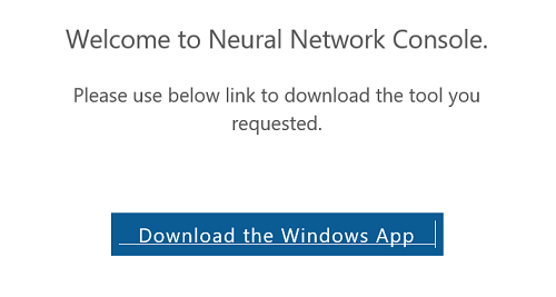
”Neural Network Console”は、Windows版と、クラウド版がありますが、もちろんGPUを活かせるWindows版をダウンロードして使います。



https://dl.sony.com

”Neural Network Console”のWindows版の最新版は”1.4.0”です。メールアドレスを登録すると、ダウンロード用のURLが記載されたメールが届くので、そこからダウンロードします。






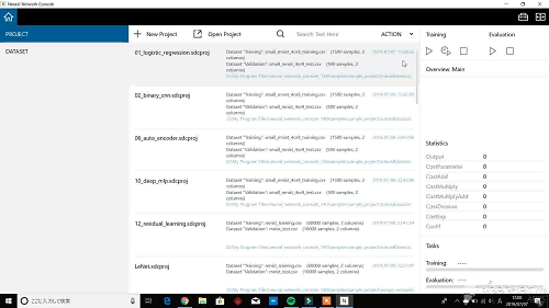
ダウンロードした、”neural_network_console_140.zip” ファイルを解凍するとと ”neural_network_console_140” フォルダの下に、"neural_network_console.exe" があるので、それを起動します。





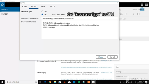
プロセッサーの設定をします。メニューのセットアップをクリックして、”ENGINE” メニューの ”Processor Type” をGPUに設定します。





”EDIT”を押すと、ニューラルネットワークのプロジェクト画面が出てきます。





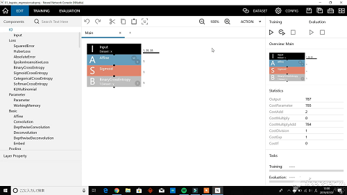
この画面の "Training" の再生ボタン（三角ボタン）を押すと学習が開始されるはずですが、なんと "`status == CUDNN_STATUS_SUCCESS`:NOT INITIALIZED" というエラーが出てしまいました。
トホホ…





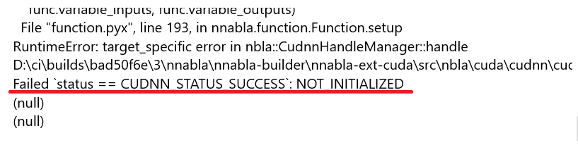
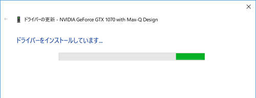
いろいろと試行錯誤をしましたが、なんのことはないディスプレイアダプタのドライバをアップデートすることで問題が解決できました。





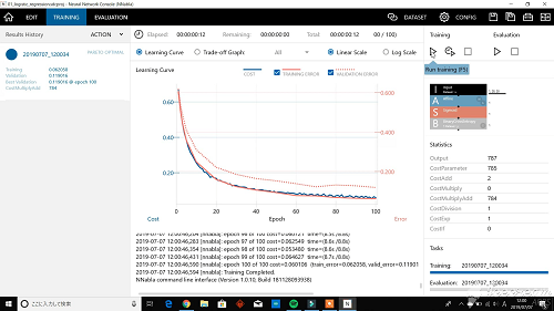
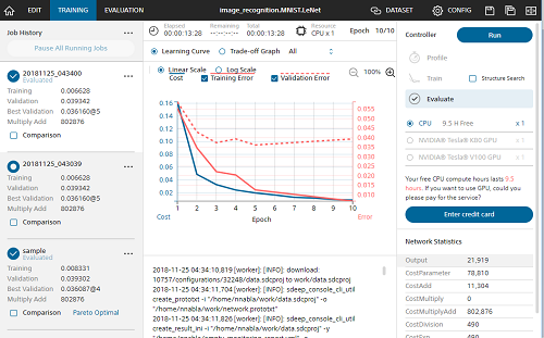
学習が終わると学習経過がグラフで表示されます。





次にプロジェクト画面の "Evalution" の再生ボタン（三角ボタン）を押すと、学習したニューラルネットワークの評価ができます。評価結果はこのニューラルネットの場合、"0" に近いと "4"、"1" に近いと "9" になります。





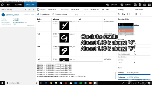
これでは、どれくらいの認識率かよくわからないので統計画面で確認します。





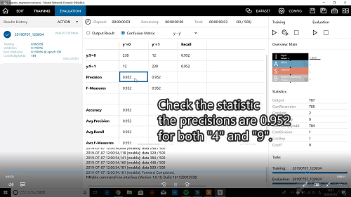
統計結果を見ると、認識率は "0.952" になりました。

さて、これをどう使うかですが、同じくソニーから出ている "SPRESENSE" で活用できます。次は、”Neural Network Console” と "SPRESENSE" の連携について試してみたいと思います。
（＾＾）／～

---

【Geforce GTX1070 with MAX-Q 搭載】OMEN by HP 15 ゲーミングノートPC 15.6インチワイド・フルHD非光沢・IPSディスプレイ Core i7-8750H Core i7-8750H メモリ16GB 256GB SSD + 2TB HDD 高速無線LAN IEEE802.11ac/a/b/g/n Bluetooth 4ZONE LEDライティング対応 日本語配列・テンキー付 バックライトキーボード Windows 10Pro 64bit シャドウブラック / ドラゴンレッド

• 出版社/メーカー: hp
• メディア:

ソニー開発のNeural Network Console入門【増補改訂・クラウド対応版】--数式なし、コーディングなしのディープラーニング

• 作者: 足立 悠
• 出版社/メーカー: リックテレコム
• 発売日: 2018/11/14
• メディア: 単行本（ソフトカバー）

---

タグ：Neural Network Console GTX1070 HP omen

自分用ノートPCを買い替え！ Deep Learning 対応へ！

長年使ってきた自分用のノートPCをついにアップデートすることにしました。最近は、IMEが時々反応しなくなったり、いつまで経ってもアプリが起動しなかったり、とっても不便でした。ブログの更新がままらない理由の一つだったりします。





新しいPCの条件は、次の３点。

　(1) Deep Learning もこなせるGPU付のマシン
　(2) 持ち運びできるサイズ
　(3) 20万円以下

いろいろ探して候補として絞り込んだのは次の２つ。


MSI GL83 8SE 070JP

MSIゲーミングノート / GL63-8SE-070JP / Core i5-8300H / GeForce RTX 2060 / メモリ16GB / SSD 256GB / HDD 1TB

• 出版社/メーカー: MSI COMPUTER
• メディア: Personal Computers

OMEN by HP 15

【Geforce GTX1070 with MAX-Q 搭載】OMEN by HP 15 ゲーミングノートPC 15.6インチワイド・フルHD非光沢・IPSディスプレイ Core i7-8750H Core i7-8750H メモリ16GB 256GB SSD + 2TB HDD 高速無線LAN IEEE802.11ac/a/b/g/n Bluetooth 4ZONE LEDライティング対応 日本語配列・テンキー付 バックライトキーボード Windows 10Pro 64bit シャドウブラック / ドラゴンレッド

• 出版社/メーカー: hp
• メディア:

GPUの性能を考えると MSI GL63SE 070JP ですが、CPU性能はOMEN by HP 15 に軍配があがります。メモリは両方 RAM16GBで、SSD256GB､その他HDDが1TBでほぼ同じです。

Model	CPU	GPU
MSI GL63 8SE	Core i5-8300H	GeForce RTX 2060
OMEN by HP 15	Core i7-8750H	GeForce GTX 1070

CPU性能は、以下の資料によると、Core i7 は Core i5 のおよそ1.5倍。（いろいろな指標がありますが、体感に近いエクセルの処理を参考にしました）


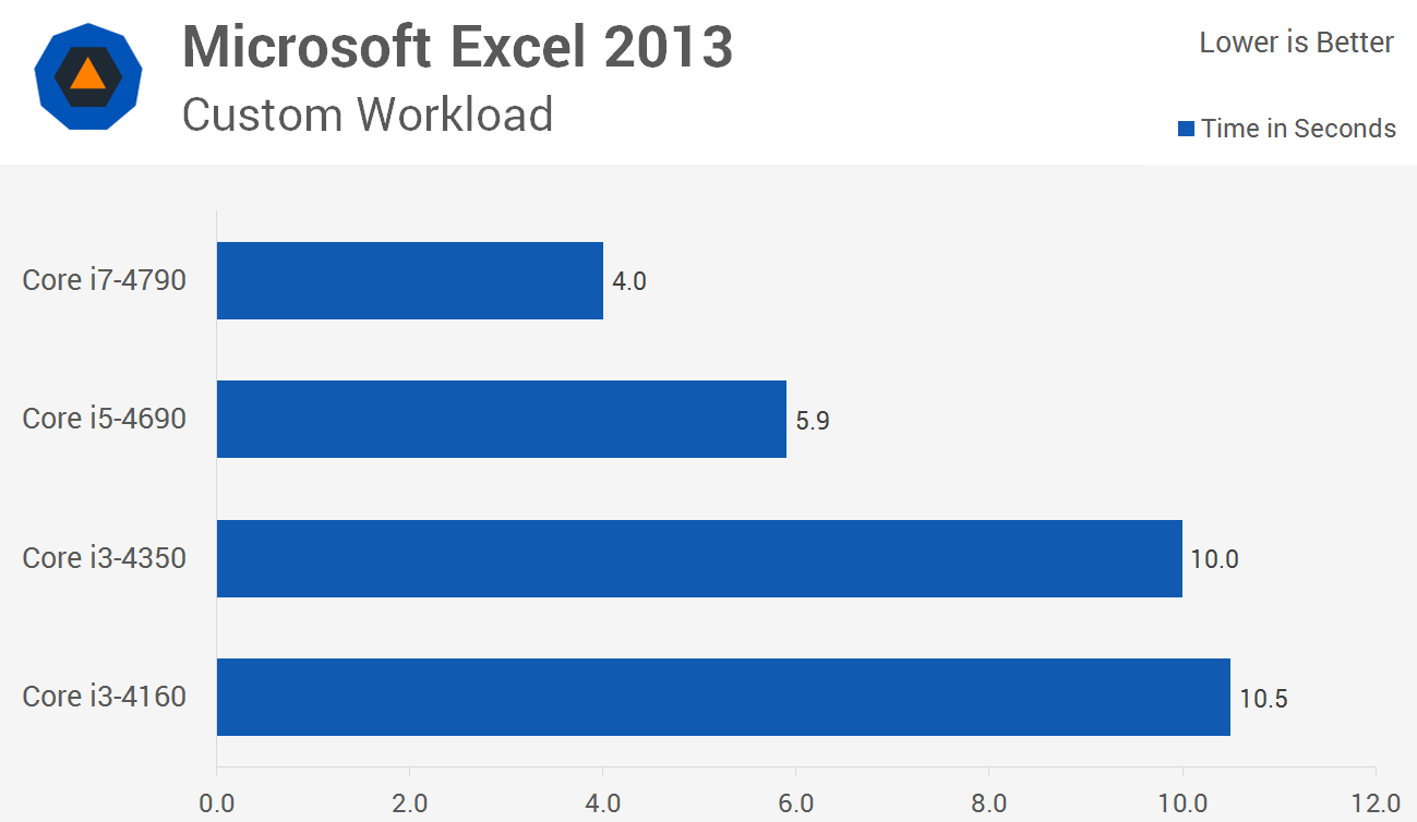
https://www.techspot.com/review/972-intel-core-i3-vs-i5-vs-i7/


GPU性能は、以下の資料によると、RTX2060 は GTX1070 のおよそ1.2倍。（こちらも、いろいろな指標がありますが、なじみのあるMonster Hunterの処理を参考にしました）


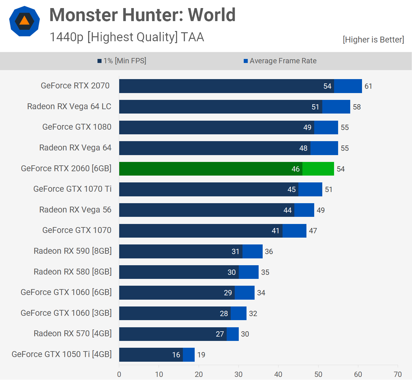
https://www.techspot.com/review/1781-geforce-rtx-2060-mega-benchmark/


製品仕様をよく比べてみると、MSI GL63SE 070JP には無線LANがついていない模様。バッテリの持ちは両方３時間程度（短い！）。重量はMSIが2.3kgで、HPが2.48kg。デザインもまぁ似たり寄ったり。

結局、CPU性能と無線LANが決定打となり、”OMEN by HP” に決めました！




ということで、このブログは OMEN by HP から書いています。いやー、快適なPCっていいですね。ただ環境の移行がめんどくさくて、一週間くらいかかりそうです。

早く Deep Learning ツールを動かしてみたいなぁ。
（＾＾）／～

---

【Geforce GTX1070 with MAX-Q 搭載】OMEN by HP 15 ゲーミングノートPC 15.6インチワイド・フルHD非光沢・IPSディスプレイ Core i7-8750H Core i7-8750H メモリ16GB 256GB SSD + 2TB HDD 高速無線LAN IEEE802.11ac/a/b/g/n Bluetooth 4ZONE LEDライティング対応 日本語配列・テンキー付 バックライトキーボード Windows 10Pro 64bit シャドウブラック / ドラゴンレッド

• 出版社/メーカー: hp
• メディア:

MSIゲーミングノート / GL63-8SE-070JP / Core i5-8300H / GeForce RTX 2060 / メモリ16GB / SSD 256GB / HDD 1TB

• 出版社/メーカー: MSI COMPUTER
• メディア: Personal Computers

Dell ゲーミングノートパソコン G5 15 5590 Core i7 ホワイト 20Q23/Win10/15.6FHD/8GB/256GB SSD+1TB HDD/GTX1650

• 出版社/メーカー: Dell Computers
• メディア: Personal Computers

タグ：OMEN by HP CPU GPU

簡単便利なソニーのディープラーニングツール！

SPRESENSEの公式ディープラーニングツールは「Neural Network Console」。ソニーから出ている”数式なし、コーディングなし”で使えるディープラーニングツールです。



https://dl.sony.com/


前回、ディープラーニングを学ぼうと、TensorFlow を始めてみましたが、Python にあまり馴染みのない私には、なんとも面倒。



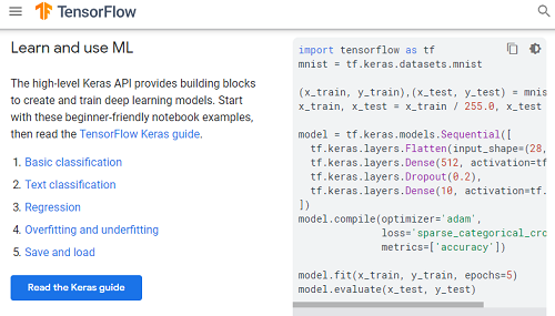
https://www.tensorflow.org/overview


でも、「Neural Network Console」ならグラフィカルにディープラーニングを構築することができます。





これなら、ディープラーニング素人の私にも出来そうな気がしてきます。統計情報も図表で示してくれて、なんか楽しく学習できそうです。





クラウド版と、無料のWinodws版があるようです。前回、PCの能力不足でTensorFlowのチュートリアルさえ動かせなかった私としてはクラウド版があるのは嬉しいところ。



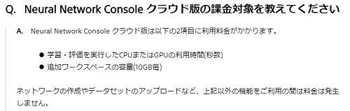
https://support.dl.sony.com/faq-ja/


クラウド版は10時間の計算時間は無料で使えるようなので、お試しに使うには十分ですね。

これから「Neural Network Console」を学習していきたいと思います！
（＾＾）／~

---

ソニー開発のNeural Network Console入門【増補改訂・クラウド対応版】--数式なし、コーディングなしのディープラーニング

• 作者: 足立 悠
• 出版社/メーカー: リックテレコム
• 発売日: 2018/11/14
• メディア: 単行本（ソフトカバー）

TensorFlowではじめるDeepLearning実装入門 (impress top gear)

• 作者: 新村 拓也
• 出版社/メーカー: インプレス
• 発売日: 2018/02/16
• メディア: 単行本（ソフトカバー）

ゼロから作るDeep Learning ―Pythonで学ぶディープラーニングの理論と実装

• 作者: 斎藤 康毅
• 出版社/メーカー: オライリージャパン
• 発売日: 2016/09/24
• メディア: 単行本（ソフトカバー）

---

タグ：Deep Learning AI

TensorFlow Deep MNIST for Experts をやってみた（２）

TensorFlow Deep MNIST for Experts のコードを動かしてみるもハングしてしまった件、問題となるコードの場所は分かりました。

def main(_):
 ... snip ...
  with tf.Session() as sess:
    sess.run(tf.global_variables_initializer())
    for i in range(1000):             #### Change step from 20000 to 1000  ####
      batch = mnist.train.next_batch(50)
      if i % 100 == 0:
        train_accuracy = accuracy.eval(feed_dict={
            x: batch[0], y_: batch[1], keep_prob: 1.0})
        print('step %d, training accuracy %g' % (i, train_accuracy))
      train_step.run(feed_dict={x: batch[0], y_: batch[1], keep_prob: 0.5})

    ### ここで問題発生！ ####
    print('test accuracy %g' % accuracy.eval(feed_dict={
        x: mnist.test.images, y_: mnist.test.labels, keep_prob: 1.0}))  

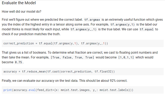
学習ステップを1000回にしてもハングしますので、ここの処理に問題がありそうです。accuracy というオブジェクトの定義を探してみたらありました。

  with tf.name_scope('accuracy'):
    correct_prediction = tf.equal(tf.argmax(y_conv, 1), tf.argmax(y_, 1)) 
    correct_prediction = tf.cast(correct_prediction, tf.float32)
  accuracy = tf.reduce_mean(correct_prediction)

argmax はそのレイヤーでの最大値のインデックスを返す関数だったはず。ということは、y_convの値と 教師データの y_ のインデックス一致しているか見ているようです。

y_conv はどうやって生成されているかというと、deepnn すなわち定義されたディープニューラルネットワークの出力です。

  # Create the model
  x = tf.placeholder(tf.float32, [None, 784])

  # Define loss and optimizer
  y_ = tf.placeholder(tf.float32, [None, 10])

  # Build the graph for the deep net
  y_conv, keep_prob = deepnn(x)

ここの一連の処理の分かりやすい解説がありました。



MNIST には、教師データとテストデータがあります。教師データは Deep Learning をしているときに使うデータ。テストデータは、Deep Learning の結果を検証するためのデータです。

ハングアップしているコードを再確認します。

    ### ここで問題発生！ ####
    print('test accuracy %g' % accuracy.eval(feed_dict={
        x: mnist.test.images, y_: mnist.test.labels, keep_prob: 1.0}))  

feed_dict は、placeholder という変数に与えるデータを置き換えるしくみです。すなわち x を mnist_test_images に、y_ を minst_test_labels に、keep_prob は 1.0 にして deepnn に突っ込んでいます。feed_dect の詳細はこちらのサイトが分かりやすかったです。


たった一行のコードですが、ここは精度を計算するために、MNIST のテストデータを deepnn に入力し y_conv を生成し、教師データと照合する処理をしています。

ということは、このテストデータの認識処理でハングしているみたいですね。うーん、明らかにPCのスペック不足ですねぇ。これは困りました。
(´・ω・`)

---

初めてのTensorFlow 数式なしのディープラーニング

• 作者: 足立 悠
• 出版社/メーカー: リックテレコム
• 発売日: 2017/10/27
• メディア: 単行本（ソフトカバー）

TensorFlowはじめました　実践！最新Googleマシンラーニング (NextPublishing)

• 出版社/メーカー: インプレスR&D
• 発売日: 2016/07/29
• メディア: Kindle版

ゼロから作るDeep Learning ―Pythonで学ぶディープラーニングの理論と実装

• 作者: 斎藤 康毅
• 出版社/メーカー: オライリージャパン
• 発売日: 2016/09/24
• メディア: 単行本（ソフトカバー）

---

タグ：Python AI 機械学習 Deep Learning

TensorFlow Deep MNIST for Experts をやってみた（１）

いよいよ、Deep Learning もディープな領域に入ってきました。前回の MNIST for ML Beginners では、92% の認識率でしたが、今回の例題ではそれを 99% まで高めることができるようです。



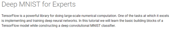
早速コードを見てみます。

# Copyright 2015 The TensorFlow Authors. All Rights Reserved.
#
# Licensed under the Apache License, Version 2.0 (the "License");
# you may not use this file except in compliance with the License.
# You may obtain a copy of the License at
#
#     http://www.apache.org/licenses/LICENSE-2.0
#
# Unless required by applicable law or agreed to in writing, software
# distributed under the License is distributed on an "AS IS" BASIS,
# WITHOUT WARRANTIES OR CONDITIONS OF ANY KIND, either express or implied.
# See the License for the specific language governing permissions and
# limitations under the License.
# ==============================================================================

"""A deep MNIST classifier using convolutional layers.
See extensive documentation at
https://www.tensorflow.org/get_started/mnist/pros
"""
# Disable linter warnings to maintain consistency with tutorial.
# pylint: disable=invalid-name
# pylint: disable=g-bad-import-order

from __future__ import absolute_import
from __future__ import division
from __future__ import print_function

import argparse
import sys
import tempfile
import os
os.environ['TF_CPP_MIN_LOG_LEVEL']='2'


from tensorflow.examples.tutorials.mnist import input_data

import tensorflow as tf

FLAGS = None


def deepnn(x):
  """deepnn builds the graph for a deep net for classifying digits.
  Args:
    x: an input tensor with the dimensions (N_examples, 784), where 784 is the
    number of pixels in a standard MNIST image.
  Returns:
    A tuple (y, keep_prob). y is a tensor of shape (N_examples, 10), with values
    equal to the logits of classifying the digit into one of 10 classes (the
    digits 0-9). keep_prob is a scalar placeholder for the probability of
    dropout.
  """
  # Reshape to use within a convolutional neural net.
  # Last dimension is for "features" - there is only one here, since images are
  # grayscale -- it would be 3 for an RGB image, 4 for RGBA, etc.
  with tf.name_scope('reshape'):
    x_image = tf.reshape(x, [-1, 28, 28, 1])

  # First convolutional layer - maps one grayscale image to 32 feature maps.
  with tf.name_scope('conv1'):
    W_conv1 = weight_variable([5, 5, 1, 32])
    b_conv1 = bias_variable([32])
    h_conv1 = tf.nn.relu(conv2d(x_image, W_conv1) + b_conv1)

  # Pooling layer - downsamples by 2X.
  with tf.name_scope('pool1'):
    h_pool1 = max_pool_2x2(h_conv1)

  # Second convolutional layer -- maps 32 feature maps to 64.
  with tf.name_scope('conv2'):
    W_conv2 = weight_variable([5, 5, 32, 64])
    b_conv2 = bias_variable([64])
    h_conv2 = tf.nn.relu(conv2d(h_pool1, W_conv2) + b_conv2)

  # Second pooling layer.
  with tf.name_scope('pool2'):
    h_pool2 = max_pool_2x2(h_conv2)

  # Fully connected layer 1 -- after 2 round of downsampling, our 28x28 image
  # is down to 7x7x64 feature maps -- maps this to 1024 features.
  with tf.name_scope('fc1'):
    W_fc1 = weight_variable([7 * 7 * 64, 1024])
    b_fc1 = bias_variable([1024])

    h_pool2_flat = tf.reshape(h_pool2, [-1, 7*7*64])
    h_fc1 = tf.nn.relu(tf.matmul(h_pool2_flat, W_fc1) + b_fc1)

  # Dropout - controls the complexity of the model, prevents co-adaptation of
  # features.
  with tf.name_scope('dropout'):
    keep_prob = tf.placeholder(tf.float32)
    h_fc1_drop = tf.nn.dropout(h_fc1, keep_prob)

  # Map the 1024 features to 10 classes, one for each digit
  with tf.name_scope('fc2'):
    W_fc2 = weight_variable([1024, 10])
    b_fc2 = bias_variable([10])

    y_conv = tf.matmul(h_fc1_drop, W_fc2) + b_fc2
  return y_conv, keep_prob


def conv2d(x, W):
  """conv2d returns a 2d convolution layer with full stride."""
  return tf.nn.conv2d(x, W, strides=[1, 1, 1, 1], padding='SAME')


def max_pool_2x2(x):
  """max_pool_2x2 downsamples a feature map by 2X."""
  return tf.nn.max_pool(x, ksize=[1, 2, 2, 1],
                        strides=[1, 2, 2, 1], padding='SAME')


def weight_variable(shape):
  """weight_variable generates a weight variable of a given shape."""
  initial = tf.truncated_normal(shape, stddev=0.1)
  return tf.Variable(initial)


def bias_variable(shape):
  """bias_variable generates a bias variable of a given shape."""
  initial = tf.constant(0.1, shape=shape)
  return tf.Variable(initial)


def main(_):
  # Import data
  mnist = input_data.read_data_sets(FLAGS.data_dir, one_hot=True)

  # Create the model
  x = tf.placeholder(tf.float32, [None, 784])

  # Define loss and optimizer
  y_ = tf.placeholder(tf.float32, [None, 10])

  # Build the graph for the deep net
  y_conv, keep_prob = deepnn(x)

  with tf.name_scope('loss'):
    cross_entropy = tf.nn.softmax_cross_entropy_with_logits(labels=y_,
                                                            logits=y_conv)
  cross_entropy = tf.reduce_mean(cross_entropy)

  with tf.name_scope('adam_optimizer'):
    train_step = tf.train.AdamOptimizer(1e-4).minimize(cross_entropy)

  with tf.name_scope('accuracy'):
    correct_prediction = tf.equal(tf.argmax(y_conv, 1), tf.argmax(y_, 1))
    correct_prediction = tf.cast(correct_prediction, tf.float32)
  accuracy = tf.reduce_mean(correct_prediction)

  graph_location = tempfile.mkdtemp()
  print('Saving graph to: %s' % graph_location)
  train_writer = tf.summary.FileWriter(graph_location)
  train_writer.add_graph(tf.get_default_graph())

  with tf.Session() as sess:
    sess.run(tf.global_variables_initializer())
    for i in range(20000):
      batch = mnist.train.next_batch(50)
      if i % 100 == 0:
        train_accuracy = accuracy.eval(feed_dict={
            x: batch[0], y_: batch[1], keep_prob: 1.0})
        print('step %d, training accuracy %g' % (i, train_accuracy))
      train_step.run(feed_dict={x: batch[0], y_: batch[1], keep_prob: 0.5})

    print('test accuracy %g' % accuracy.eval(feed_dict={
        x: mnist.test.images, y_: mnist.test.labels, keep_prob: 1.0}))

if __name__ == '__main__':
  parser = argparse.ArgumentParser()
  parser.add_argument('--data_dir', type=str,
                      default='/tmp/tensorflow/mnist/input_data',
                      help='Directory for storing input data')
  FLAGS, unparsed = parser.parse_known_args()
  tf.app.run(main=main, argv=[sys.argv[0]] + unpars

前回よりかなり複雑になってますね。実行をしてみたのですが、何度やっても9900回目くらいでPCがハングアップしてしまいます。学習もかなり時間がかかってしまいますし、仕方ないので学習ステップを 5000回くらいに変更しました。

.... snip ...
def main(_):
  # Import data
  mnist = input_data.read_data_sets(FLAGS.data_dir, one_hot=True)

 ... snip ...
  with tf.Session() as sess:
    sess.run(tf.global_variables_initializer())
    for i in range(5000):             #### Change step from 20000 to 5000  ####
      batch = mnist.train.next_batch(50)
      if i % 100 == 0:
        train_accuracy = accuracy.eval(feed_dict={
            x: batch[0], y_: batch[1], keep_prob: 1.0})
        print('step %d, training accuracy %g' % (i, train_accuracy))
      train_step.run(feed_dict={x: batch[0], y_: batch[1], keep_prob: 0.5})

    print('test accuracy %g' % accuracy.eval(feed_dict={
        x: mnist.test.images, y_: mnist.test.labels, keep_prob: 1.0}))

これでうまく行くかと思ったのですが、4900回が終わったところでまたPCがハングしてしまいました。
(´；ω；｀)

タスクマネージャーを立ち上げながら処理の様子を見てみたら、終了処理のところで大量のメモリを確保にいき、メモリ不足が発生してハングしてしまっているようです。(正確には大量のスワップが発生し、HDDの帯域不足が発生したものと思います)

4GBメモリ + HDD のノートパソコンじゃ Deep Learning ムリってこと？困ったなぁ。おいおい解析していきたいと思います。
(´・ω・｀)

---

初めてのTensorFlow 数式なしのディープラーニング

• 作者: 足立 悠
• 出版社/メーカー: リックテレコム
• 発売日: 2017/10/27
• メディア: 単行本（ソフトカバー）

TensorFlowはじめました　実践！最新Googleマシンラーニング (NextPublishing)

• 出版社/メーカー: インプレスR&D
• 発売日: 2016/07/29
• メディア: Kindle版

ゼロから作るDeep Learning ―Pythonで学ぶディープラーニングの理論と実装

• 作者: 斎藤 康毅
• 出版社/メーカー: オライリージャパン
• 発売日: 2016/09/24
• メディア: 単行本（ソフトカバー）

---

タグ：機械学習 Deep Learning Tensorflow Python AI

TensorFlow MNIST For ML Beginners をやってみた（２）

TensorFlow MNIST For ML Beginners をやってみると使い方はわかりますが、理屈がわからないと気持ち悪いですよね。少し TensorFlow から話ははずれますが、Deep Learning の理屈について考えてみます。

ポイントは、損失関数と学習の仕組みです。損失関数を最小にするように学習するというのが Deep Learning の理屈ですが、これは蓋を開けてみると、最小二乗法で近似曲線を割り出す理屈と同じだったりします。


こちらのページが最も分かりやすかったです。

解けない連立方程式とディープラーニング
http://www.fward.net/archives/2126


ここで、上のサイトでサンプルに出ている行列を考えてみます。これは MNIST のミニチュア版といえます。





ここで、重みデータであるWを変数、損失関数を二乗誤差とすると二次曲線で表せます。このWの値を曲線の傾きに学習係数ηを掛けた分だけずらしていき、損失関数が最小になる曲率ゼロまで近づけていきます。





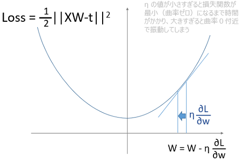
この学習係数ηは、結構くせもので図を見てもわかるように、小さすぎると学習ステップを多くしなければならないですし、大きすぎると曲率ゼロ付近で振動をしてしまいます。

さて理屈は分かったのですが、せっかくなのでプログラムを作って検証したいところです。そこで損失関数の微分値の式を導出してみましょう。行列の微分なのでちょっとやっかいです。

最初に損失関数を展開します。絶対値なので、転置行列と行列の積になることに注意します。





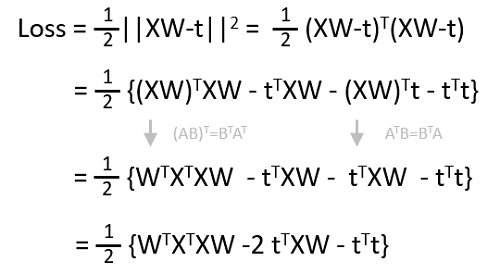
さて、微分をしてみましょう。行列の微分には公式があります。こちらのサイトがよくまとまっています。





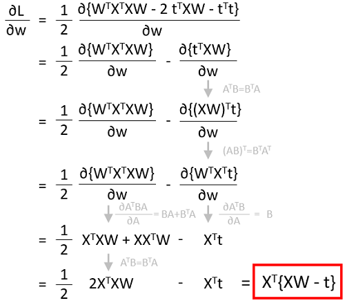
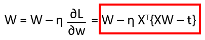
ということで損失関数の微分は、Xの転置行列に教師データと計算値の誤差を掛けたものになりました。





それにηをかけてWの値を更新します。





これを python のプログラムにしてみました。η は 0.0229 と設定しています。

import numpy as np
import math

X = np.array([[1,1], [3,1], [5,1], [7,1]], dtype="float").reshape((4, 2))
w = np.array([1, 1], dtype="float").reshape((2,1))
t = np.array([1, 4, 4, 8], dtype="float").reshape((4,1))

L = np.dot(X,w) - t  # X*w - t
Loss = (sum(np.power(L,2))/2).round(8)  # ||X*W - t||^2 / 2
preLoss = Loss
print(Loss)

eta = 0.0229
for i in range(5000):
   dL = np.dot(X.T,(np.dot(X,w) - t))  # XT*{XW - t}
   w = w - np.dot(eta,dL)  # W = W - eta*dL/dw
   L = np.dot(X,w) - t
   Loss = (sum(np.power(L,2))/2).round(8)
   if preLoss <= Loss:
       break;
   preLoss = Loss
   print(Loss)

print(i)
print(Loss)
print(w)

これを実行すると以下のようになります。

1174
[ 1.35000079]
[[ 1.04986813]
 [ 0.0499746 ]]

1174回目で損失関数が最小になり、値は1.35。Wa は 1.05、Wb は 0.05 になりました。解説サイトの数値とあっていますね。

これで、学習の実態はわかりました。損失関数や学習ステップ、学習係数が把握できたところで次のステップに進みますか。あーすっきりした。
(*^_^*)

---

ゼロから作るDeep Learning ―Pythonで学ぶディープラーニングの理論と実装

• 作者: 斎藤 康毅
• 出版社/メーカー: オライリージャパン
• 発売日: 2016/09/24
• メディア: 単行本（ソフトカバー）

ディープラーニングがわかる数学入門

• 作者: 涌井 良幸
• 出版社/メーカー: 技術評論社
• 発売日: 2017/03/28
• メディア: 単行本（ソフトカバー）

TensorFlowはじめました　実践！最新Googleマシンラーニング (NextPublishing)

• 出版社/メーカー: インプレスR&D
• 発売日: 2016/07/29
• メディア: Kindle版

---

タグ：Deep Learning AI 機械学習 Python

TensorFlow MNIST For ML Beginners をやってみた（１）

TensorFlow でいよいよ認識処理を試してみたいと思います。ニューラルネットワークの基本中の基本である手書き文字の認識が例題です。





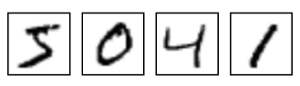
MNIST とは、その手書き文字を学習させるためのデータセットのことです。（MLとは Machine Learning のことです）例えばこんなデータが訓練用に6万点、テスト用に1万点、用意されています。





MNISTのデータは Yann LeCun's website からダウンロードすることができます。ダウンロードしてくるファイルは４種類あります。

train-images-idx3-ubyte.gz
train-labels-idx1-ubyte.gz
t10k-images-idx3-ubyte.gz
t10k-labels-idx1-ubyte.gz

これらをダウンロードしたら、MNIST_data というディレクトリを作って格納しておきます。解凍は必要はありません。


Deep Learning用のテストプログラムを用意します。TensorFlow GitHub Site からもダウンロードできます。

# Copyright 2015 The TensorFlow Authors. All Rights Reserved.
#
# Licensed under the Apache License, Version 2.0 (the "License");
# you may not use this file except in compliance with the License.
# You may obtain a copy of the License at
#
#     http://www.apache.org/licenses/LICENSE-2.0
#
# Unless required by applicable law or agreed to in writing, software
# distributed under the License is distributed on an "AS IS" BASIS,
# WITHOUT WARRANTIES OR CONDITIONS OF ANY KIND, either express or implied.
# See the License for the specific language governing permissions and
# limitations under the License.
# ==============================================================================

"""A very simple MNIST classifier.
See extensive documentation at
https://www.tensorflow.org/get_started/mnist/beginners
"""
from __future__ import absolute_import
from __future__ import division
from __future__ import print_function

import argparse
import sys
import os
os.environ['TF_CPP_MIN_LOG_LEVEL']='2'

from tensorflow.examples.tutorials.mnist import input_data

import tensorflow as tf

FLAGS = None


def main(_):
  # Import data
  mnist = input_data.read_data_sets(FLAGS.data_dir, one_hot=True)

  # Create the model
  x = tf.placeholder(tf.float32, [None, 784])
  W = tf.Variable(tf.zeros([784, 10]))
  b = tf.Variable(tf.zeros([10]))
  y = tf.matmul(x, W) + b

  # Define loss and optimizer
  y_ = tf.placeholder(tf.float32, [None, 10])

  # The raw formulation of cross-entropy,
  #
  #   tf.reduce_mean(-tf.reduce_sum(y_ * tf.log(tf.nn.softmax(y)),
  #                                 reduction_indices=[1]))
  #
  # can be numerically unstable.
  #
  # So here we use tf.nn.softmax_cross_entropy_with_logits on the raw
  # outputs of 'y', and then average across the batch.
  cross_entropy = tf.reduce_mean(
      tf.nn.softmax_cross_entropy_with_logits(labels=y_, logits=y))
  train_step = tf.train.GradientDescentOptimizer(0.5).minimize(cross_entropy)

  sess = tf.InteractiveSession()
  tf.global_variables_initializer().run()
  # Train
  for _ in range(1000):
    batch_xs, batch_ys = mnist.train.next_batch(100)
    sess.run(train_step, feed_dict={x: batch_xs, y_: batch_ys})

  # Test trained model
  correct_prediction = tf.equal(tf.argmax(y, 1), tf.argmax(y_, 1))
  accuracy = tf.reduce_mean(tf.cast(correct_prediction, tf.float32))
  print(sess.run(accuracy, feed_dict={x: mnist.test.images,
                                      y_: mnist.test.labels}))

if __name__ == '__main__':
  parser = argparse.ArgumentParser()
  parser.add_argument('--data_dir', type=str, default='/tmp/tensorflow/mnist/input_data',
                      help='Directory for storing input data')
  FLAGS, unparsed = parser.parse_known_args()
  tf.app.run(main=main, argv=[sys.argv[0]] + unparsed)

実際に動かしてみました。

C:\Users\Taro\Documents\TensorFlow>python mnist_softmax.py --data_dir MNIST_data
Extracting MNIST_data\train-images-idx3-ubyte.gz
Extracting MNIST_data\train-labels-idx1-ubyte.gz
Extracting MNIST_data\t10k-images-idx3-ubyte.gz
Extracting MNIST_data\t10k-labels-idx1-ubyte.gz
0.9206

素っ気ない結果ですね。何をしているかはソースコードを読み解くしかありません。大きな処理の流れは以下になります。

（１）MNISTデータを読み込み
（２）ニューラルネットワークの数式モデルを定義
（３）損失関数を設定
（４）学習データでネットワークを学習
（５）テストデータで結果を確認

という感じです。それぞれのコードを抜粋すると以下になります。


（１）MNISTデータの読み込み

mnist = input_data.read_data_sets(FLAGS.data_dir, one_hot=True)

最後の one_hot というのは、一つの正解だけが１でその他は0となるような設定のことです。


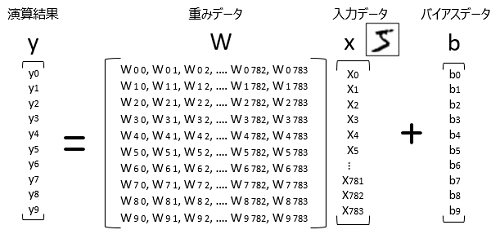
（２）ニューラルネットワークの数式モデルを定義

  x = tf.placeholder(tf.float32, [None, 784])
  W = tf.Variable(tf.zeros([784, 10]))
  b = tf.Variable(tf.zeros([10]))
  y = tf.matmul(x, W) + b

784 x 10 の配列が定義されていますが、これは、28pixel x 28pixel = 784 pixel の文字データ、0-9 の10個のデータを示しています。x は手書きデータの入力で、bはバイアス、yはその出力です。




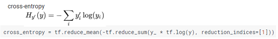
（３）損失関数を設定

cross_entropy = tf.reduce_mean( tf.nn.softmax_cross_entropy_with_logits(labels=y_, logits=y))

このニューラルネットワークの判定には、softmax 関数というものを使います。



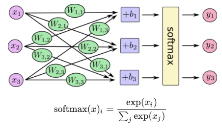
詳細の理屈は抜きにして、この場合、損失関数には cross_entropy という関数を使います。




（４）学習データでネットワークを学習

 for _ in range(1000):
    batch_xs, batch_ys = mnist.train.next_batch(100)
    sess.run(train_step, feed_dict={x: batch_xs, y_: batch_ys})

ここで batch というものが出てきました。この場合は100個データの損失関数を算出してその平均を学習用の損失データとして扱うという処理方法の様です。学習のための計算量を減らすことができると考えておけばよさそうです。


（５）テストデータで結果を確認

correct_prediction = tf.equal(tf.argmax(y, 1), tf.argmax(y_, 1))
accuracy = tf.reduce_mean(tf.cast(correct_prediction, tf.float32))
print(sess.run(accuracy, feed_dict={x: mnist.test.images, y_: mnist.test.labels}))

argmax(y, 1) というのはy行列の中から最大値を一つだけ抽出するというものです。yの計算結果と、 softmax の計算結果 y_ があっているかどうかで判定し、その判定結果の平均値から検出率を算出しています。

例えば、判定結果が [True,True,True,False,True,True,True,False,True,True] だとすると、検出率は0.8ということになります。


なんとなく処理の内容は見えてきました。次はどうやって学習しているのか詳しく見ていきたいと思います。しかし、行列演算のオンパレードで難しいなぁ。
σ（ー_ ー；

---

TensorFlowはじめました　実践！最新Googleマシンラーニング (NextPublishing)

• 出版社/メーカー: インプレスR&D
• 発売日: 2016/07/29
• メディア: Kindle版

ゼロから作るDeep Learning ―Pythonで学ぶディープラーニングの理論と実装

• 作者: 斎藤 康毅
• 出版社/メーカー: オライリージャパン
• 発売日: 2016/09/24
• メディア: 単行本（ソフトカバー）

TensorFlow機械学習クックブック Pythonベースの活用レシピ60+ (impress top gear)

• 作者: Nick McClure
• 出版社/メーカー: インプレス
• 発売日: 2017/08/14
• メディア: 単行本（ソフトカバー）

---

タグ：Python AI 機械学習 Tensorflow Deep Learning

TensorFlow Core tutorial を学んでみた（３）～ tf.estimator～

TensorFlow Core tutorial も今回で最後です。Estimator というものを使ってみました。



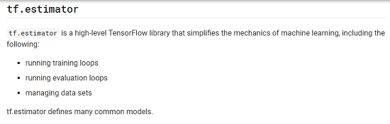
https://www.tensorflow.org/get_started/get_started#tfestimator


うーん、正直よく分からないのですが、損失関数が最小になるように条件を求め、かつそれを評価するためのツールといったところでしょうか？

とりあえずコードを見よう見まねで書いてみました。Basic Usage と A custom model の二つがありますが、A custom model のほうが見通しがよいので試してみました。

import os
os.environ['TF_CPP_MIN_LOG_LEVEL']='2'
import tensorflow as tf
import numpy as np

# delare list of features, 
def model_fn(features, labels, mode):
    # Build a linear model 
    W = tf.get_variable("W", [1], dtype=tf.float64)
    b = tf.get_variable("b", [1], dtype=tf.float64)
    y = W * features['x'] + b
    loss = tf.reduce_sum(tf.square(y - labels))

    # training to minimize loss
    global_step = tf.train.get_global_step()
    optimizer   = tf.train.GradientDescentOptimizer(0.01)
    train = tf.group(optimizer.minimize(loss), tf.assign_add(global_step, 1))

    return tf.estimator.EstimatorSpec(mode=mode ,predictions=y 
            ,loss=loss ,train_op=train)


estimator = tf.estimator.Estimator(model_fn=model_fn)

# defin data sets
x_train = np.array([ 1.0 , 2.0 , 3.0 , 4.0])
y_train = np.array([ 0.0 ,-1.0 ,-2.0 ,-3.0])
x_eval  = np.array([ 2.0 , 5.0 , 8.0 , 1.0])
y_eval  = np.array([-1.01,-4.1 ,-7.0 , 0.0])

input_fn       = tf.estimator.inputs.numpy_input_fn(
        {"x": x_train} ,y_train ,batch_size=4 ,num_epochs=None ,shuffle=True)

train_input_fn = tf.estimator.inputs.numpy_input_fn(
        {"x": x_train} ,y_train ,batch_size=4 ,num_epochs=1000 ,shuffle=False)

eval_input_fn  = tf.estimator.inputs.numpy_input_fn(
        {"x": x_eval } ,y_eval  ,batch_size=4 ,num_epochs=1000 ,shuffle=False)

# train
estimator.train(input_fn=input_fn ,steps=1000)

# evaluate the model defined
train_metrics = estimator.evaluate(input_fn=train_input_fn)
eval_metrics  = estimator.evaluate(input_fn=eval_input_fn)
print("train metrics: %r"% train_metrics)
print("eval  metrics: %r"% eval_metrics)

実行結果がこちら。

C:\Users\Taro\Documents\TensorFlow>python estimator.py
WARNING:tensorflow:Using temporary folder as model directory: C:\Users\Taro\AppData\Local\Temp\tmp_ad4se
train metrics: {'global_step': 1000, 'loss': 1.265121e-11}
eval  metrics: {'global_step': 1000, 'loss': 0.010100436}

うーん、たしかにlossが小さくなるようになったようです。Eval は実際のデータで試してみた値なのかな。説明がほとんどないのでよく分かりません。

とりあえず、わざわざループを作らなくても損失関数を最小にできる便利なツールがある程度で理解して先に進もうと思います。
σ（ー_ ー;）ワカラン

---

TensorFlowはじめました　実践！最新Googleマシンラーニング (NextPublishing)

• 出版社/メーカー: インプレスR&D
• 発売日: 2016/07/29
• メディア: Kindle版

ゼロから作るDeep Learning ―Pythonで学ぶディープラーニングの理論と実装

• 作者: 斎藤 康毅
• 出版社/メーカー: オライリージャパン
• 発売日: 2016/09/24
• メディア: 単行本（ソフトカバー）

TensorFlow機械学習クックブック Pythonベースの活用レシピ60+ (impress top gear)

• 作者: Nick McClure
• 出版社/メーカー: インプレス
• 発売日: 2017/08/14
• メディア: 単行本（ソフトカバー）

---

タグ：Deep Learning AI 機械学習 Tensorflow Python

TensorFlow Core tutorial を学んでみた（２）～ tf.train API～

TensorFlow の Core tutorial で紹介されている train API について学んでみました。


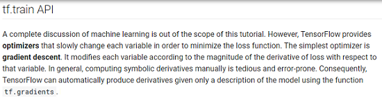
https://www.tensorflow.org/get_started/get_started#tftrain_api

train API は、損失関数である差分二乗和を最小する係数を求めていくための関数です。前回、以下の関数を考えてみました。

x = [1, 2, 3, 4]
y = [0, -1, -2, -3]
squared_deltas = (W * x + b) - y) * ((W * x + b) - y )
loss = SUM(squared_deltas)

この時に、与えられた x, y の値から loss が最小となるように W と b の値をかえていくのが train API の機能です。いくつか手法があるようですが、Core tutorial では Gradient Descent (勾配降下法) が使われています。

引数は学習係数(learning rate)で、この数値を変えることで学習速度が変わるようです。学習の様子を確認するためのサンプルコードを作ってみました。

import os
os.environ['TF_CPP_MIN_LOG_LEVEL']='2'
import tensorflow as tf

# define variables with initial value
W = tf.Variable([0.3], dtype=tf.float32)
b = tf.Variable([-0.3], dtype=tf.float32)

# Model input and output
x = tf.placeholder(tf.float32)
linear_model = W * x + b
y = tf.placeholder(tf.float32)

# loss
loss = tf.reduce_sum(tf.square(linear_model - y))

# set learning rate to gradient decent optimizer
learning_rate = 0.01
print("learning rate: %s"%learning_rate)
optimizer = tf.train.GradientDescentOptimizer(learning_rate)
train = optimizer.minimize(loss)

# training data
x_train = [1, 2, 3, 4]
y_train = [0, -1, -2, -3]

# traing loop
init = tf.global_variables_initializer()
sess = tf.Session()
sess.run(init)
# create exection instance
sess = tf.Session()

# initialize variables
init = tf.global_variables_initializer()
sess.run(init)

# initial
curr_W, curr_b, curr_loss = sess.run([W, b, loss], {x: x_train, y: y_train})
print("W: %s b: %s loss: %s"%(curr_W, curr_b, curr_loss))

# 1st training 
for i in range(100):
    sess.run(train, {x: x_train, y: y_train})
curr_W, curr_b, curr_loss = sess.run([W, b, loss], {x: x_train, y: y_train})
print("W: %s b: %s loss: %s"%(curr_W, curr_b, curr_loss))

# 2nd training 
for i in range(100):
    sess.run(train, {x: x_train, y: y_train})
curr_W, curr_b, curr_loss = sess.run([W, b, loss], {x: x_train, y: y_train})
print("W: %s b: %s loss: %s"%(curr_W, curr_b, curr_loss))

# 3rd training
for i in range(100):
    sess.run(train, {x: x_train, y: y_train})
curr_W, curr_b, curr_loss = sess.run([W, b, loss], {x: x_train, y: y_train})
print("W: %s b: %s loss: %s"%(curr_W, curr_b, curr_loss))

# 4th training
for i in range(100):
    sess.run(train, {x: x_train, y: y_train})
curr_W, curr_b, curr_loss = sess.run([W, b, loss], {x: x_train, y: y_train})
print("W: %s b: %s loss: %s"%(curr_W, curr_b, curr_loss))

# 5th training
for i in range(100):
    sess.run(train, {x: x_train, y: y_train})
curr_W, curr_b, curr_loss = sess.run([W, b, loss], {x: x_train, y: y_train})
print("W: %s b: %s loss: %s"%(curr_W, curr_b, curr_loss))

# 6th training
for i in range(100):
    sess.run(train, {x: x_train, y: y_train})
curr_W, curr_b, curr_loss = sess.run([W, b, loss], {x: x_train, y: y_train})
print("W: %s b: %s loss: %s"%(curr_W, curr_b, curr_loss))

# 7th training
for i in range(100):
    sess.run(train, {x: x_train, y: y_train})
curr_W, curr_b, curr_loss = sess.run([W, b, loss], {x: x_train, y: y_train})
print("W: %s b: %s loss: %s"%(curr_W, curr_b, curr_loss))

# 8th training
for i in range(100):
    sess.run(train, {x: x_train, y: y_train})
curr_W, curr_b, curr_loss = sess.run([W, b, loss], {x: x_train, y: y_train})
print("W: %s b: %s loss: %s"%(curr_W, curr_b, curr_loss))

# 9th training
for i in range(100):
    sess.run(train, {x: x_train, y: y_train})
curr_W, curr_b, curr_loss = sess.run([W, b, loss], {x: x_train, y: y_train})
print("W: %s b: %s loss: %s"%(curr_W, curr_b, curr_loss))

# 10th training
for i in range(100):
    sess.run(train, {x: x_train, y: y_train})
curr_W, curr_b, curr_loss = sess.run([W, b, loss], {x: x_train, y: y_train})
print("W: %s b: %s loss: %s"%(curr_W, curr_b, curr_loss))

学習係数を変えながら出力をしてみました。まずは係数を減らしてみます。学習係数を減らしていくとloss の減り方が緩やかになっているのが分かります。

C:\Users\Taro\Documents\TensorFlow>python trainapi.py
learning rate: 0.01
W: [ 0.30000001] b: [-0.30000001] loss: 23.66
W: [-0.84079814] b: [ 0.53192717] loss: 0.146364
W: [-0.95227844] b: [ 0.85969269] loss: 0.0131513
W: [-0.98569524] b: [ 0.95794231] loss: 0.00118168
W: [-0.99571204] b: [ 0.98739296] loss: 0.000106178
W: [-0.99871475] b: [ 0.99622124] loss: 9.5394e-06
W: [-0.99961478] b: [ 0.99886739] loss: 8.56873e-07
W: [-0.99988455] b: [ 0.99966055] loss: 7.69487e-08
W: [-0.99996537] b: [ 0.99989825] loss: 6.90848e-09
W: [-0.99998957] b: [ 0.99996936] loss: 6.24471e-10
W: [-0.9999969] b: [ 0.99999082] loss: 5.69997e-11

C:\Users\Taro\Documents\TensorFlow>python trainapi.py
learning rate: 0.005
W: [ 0.30000001] b: [-0.30000001] loss: 23.66
W: [-0.70869172] b: [ 0.14351812] loss: 0.490055
W: [-0.84021938] b: [ 0.53022552] loss: 0.14743
W: [-0.91236132] b: [ 0.74233174] loss: 0.0443537
W: [-0.95193082] b: [ 0.85867071] loss: 0.0133436
W: [-0.97363442] b: [ 0.92248183] loss: 0.00401434
W: [-0.9855386] b: [ 0.95748174] loss: 0.0012077
W: [-0.99206799] b: [ 0.97667885] loss: 0.000363336
W: [-0.99564934] b: [ 0.98720855] loss: 0.000109307
W: [-0.99761379] b: [ 0.99298412] loss: 3.2883e-05
W: [-0.9986912] b: [ 0.99615198] loss: 9.89192e-06

C:\Users\Taro\Documents\TensorFlow>python trainapi.py
learning rate: 0.001
W: [ 0.30000001] b: [-0.30000001] loss: 23.66
W: [-0.52810556] b: [-0.3849203] loss: 1.28182
W: [-0.58207232] b: [-0.22875588] loss: 1.00865
W: [-0.62926829] b: [-0.08999654] loss: 0.793704
W: [-0.67113376] b: [ 0.03309342] loss: 0.624565
W: [-0.70827162] b: [ 0.14228313] loss: 0.491469
W: [-0.74121565] b: [ 0.2391424] loss: 0.386737
W: [-0.77043933] b: [ 0.32506362] loss: 0.304323
W: [-0.796363] b: [ 0.40128195] loss: 0.239471
W: [-0.819359] b: [ 0.46889341] loss: 0.188439
W: [-0.83975828] b: [ 0.52886957] loss: 0.148283

今度は逆に係数を増やしてみました。

C:\Users\Taro\Documents\TensorFlow>python trainapi.py
learning rate: 0.01
W: [ 0.30000001] b: [-0.30000001] loss: 23.66
W: [-0.84079814] b: [ 0.53192717] loss: 0.146364
W: [-0.95227844] b: [ 0.85969269] loss: 0.0131513
W: [-0.98569524] b: [ 0.95794231] loss: 0.00118168
W: [-0.99571204] b: [ 0.98739296] loss: 0.000106178
W: [-0.99871475] b: [ 0.99622124] loss: 9.5394e-06
W: [-0.99961478] b: [ 0.99886739] loss: 8.56873e-07
W: [-0.99988455] b: [ 0.99966055] loss: 7.69487e-08
W: [-0.99996537] b: [ 0.99989825] loss: 6.90848e-09
W: [-0.99998957] b: [ 0.99996936] loss: 6.24471e-10
W: [-0.9999969] b: [ 0.99999082] loss: 5.69997e-11

C:\Users\Taro\Documents\TensorFlow>python trainapi.py
learning rate: 0.02
W: [ 0.30000001] b: [-0.30000001] loss: 23.66
W: [-0.95297438] b: [ 0.8617391] loss: 0.0127705
W: [-0.99583626] b: [ 0.98775804] loss: 0.000100119
W: [-0.9996314] b: [ 0.99891615] loss: 7.84759e-07
W: [-0.9999674] b: [ 0.99990404] loss: 6.14229e-09
W: [-0.99999708] b: [ 0.99999142] loss: 4.92442e-11
W: [-0.99999952] b: [ 0.99999869] loss: 1.06581e-12
W: [-0.99999952] b: [ 0.99999869] loss: 1.06581e-12
W: [-0.99999952] b: [ 0.99999869] loss: 1.06581e-12
W: [-0.99999952] b: [ 0.99999869] loss: 1.06581e-12
W: [-0.99999952] b: [ 0.99999869] loss: 1.06581e-12

C:\Users\Taro\Documents\TensorFlow>python trainapi.py
learning rate: 0.03
W: [ 0.30000001] b: [-0.30000001] loss: 23.66
W: [ 0.16820002] b: [ 1.35244703] loss: 49.6722
W: [ 0.73389339] b: [ 1.58857942] loss: 111.988
W: [ 1.60297251] b: [ 1.88529921] loss: 252.487
W: [ 2.90843058] b: [ 2.32934356] loss: 569.256
W: [ 4.86862707] b: [ 2.99604988] loss: 1283.44
W: [ 7.81191444] b: [ 3.9971242] loss: 2893.63
W: [ 12.23135185] b: [ 5.50027037] loss: 6523.96
W: [ 18.86728859] b: [ 7.75730085] loss: 14708.9
W: [ 28.83135033] b: [ 11.14629936] loss: 33162.6
W: [ 43.7927475] b: [ 16.23500061] loss: 74768.5

C:\Users\Taro\Documents\TensorFlow>python trainapi.py
learning rate: 0.04
W: [ 0.30000001] b: [-0.30000001] loss: 23.66
W: [  1.62939458e+22] b: [  5.54192817e+21] loss: inf
W: [ nan] b: [ nan] loss: nan
W: [ nan] b: [ nan] loss: nan
W: [ nan] b: [ nan] loss: nan
W: [ nan] b: [ nan] loss: nan
W: [ nan] b: [ nan] loss: nan
W: [ nan] b: [ nan] loss: nan
W: [ nan] b: [ nan] loss: nan
W: [ nan] b: [ nan] loss: nan
W: [ nan] b: [ nan] loss: nan

0.02までは早く収束していますが、0.03から不安定になり、0.04では発散してしまいました。制御係数と同じで値を大きくしていくと発散しやすくなるようです。

当然、モデルによって最適な学習係数は変わりますが、この値は経験値で求めるのしかないのかな。その辺りも追々調べていきたいと思います。
（＾_＾）／～

---

TensorFlowはじめました　実践！最新Googleマシンラーニング (NextPublishing)

• 出版社/メーカー: インプレスR&D
• 発売日: 2016/07/29
• メディア: Kindle版

ゼロから作るDeep Learning ―Pythonで学ぶディープラーニングの理論と実装

• 作者: 斎藤 康毅
• 出版社/メーカー: オライリージャパン
• 発売日: 2016/09/24
• メディア: 単行本（ソフトカバー）

TensorFlow機械学習クックブック Pythonベースの活用レシピ60+ (impress top gear)

• 作者: Nick McClure
• 出版社/メーカー: インプレス
• 発売日: 2017/08/14
• メディア: 単行本（ソフトカバー）

---

タグ：Deep Learning Tensorflow 機械学習 AI Python